Different Ways to Create Pandas DataFrames

A Pandas DataFrame is a 2D labeled data structure with columns of potentially different types.

There are a variety of different methods and syntaxes that can be used to create a pd.DataFrame.

Firstly, make sure you import the pandas module:

import pandas as pd

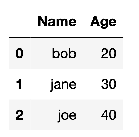
Method 1: Creating DataFrame from list of lists

# initialize list of lists
data = [['bob', 20], ['jane', 30], ['joe', 40]]
 
# Create the pandas DataFrame
df = pd.DataFrame(data, columns = ['Name', 'Age'])
df

Output:

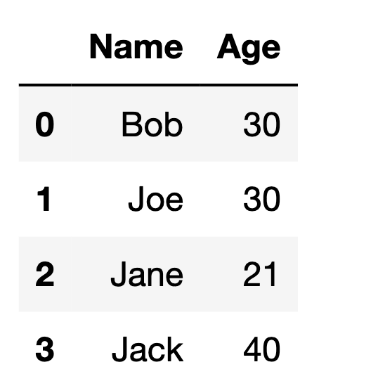
Method #2: Creating DataFrame from dictionary of lists

In this method, you define a dictionary which has the column name as the key which corresponds to an array of row values.

# initialize dictionary of lists
data = {'Name': ['Bob', 'Joe', 'Jane', 'Jack'],
        'Age': [30, 30, 21, 40]}
 
# Create DataFrame
df = pd.DataFrame(data)
df

Output:

You can use custom index values for the DataFrame by adding a parameter to the pd.DataFrame function. Set the optional index parameter of the pd.DataFrame function to an array of strings for the index values.

df = pd.DataFrame(data, index=['first',
                                'second',
                                'third',
                                'fourth'])
df

Output:

In the same way that we just defined the index values, you can also define the column names separately. Set the optional columns parameter of the pd.DataFrame function to an array of strings for the column values.

Notice that the row values are now defined as a list of lists rather than a dictionary of lists. This is because the column values are no longer being defined with them.

df = pd.DataFrame(
    [[4,5,6],
     [7,8,9],
     [10,11,12]],
    index = ['row_one','row_two','row_three'],
    columns=["a","b","c"]
    )

df

Output:

Method #3: Creating DataFrame using zip() function.

The zip function returns an iterator of tuples where the corresponding items in each passed iterator is paired together. By calling the list function on the object returned from the zip function, we convert the object to a list which can be passed into the pd.DataFrame function.

name = ["Bob", "Sam", "Sally", "Sue"]
age = [19, 17, 51, 49]

data = list(zip(name, age))

df = pd.DataFrame(data,
                  columns = ['Name', 'Age'])

df

Output:

How to Create 3-D Charts with Matplotlib in Jupyter Notebook

In this article, I will show you how to work with 3D plots in Matplotlib. Specifically, we will be making a 3D line plot and surface plot.

First, import matplotlib and numpy. %matplotlib inline just sets the backend of matplotlib to the ‘inline’ backend, so the output of plotting commands shows inline (directly below the code cell that produced it).

import matplotlib.pyplot as plt
import numpy as np

%matplotlib inline

Add this import statement to work with 3D axes in matplotlib:

from mpl_toolkits.mplot3d.axes3d import Axes3D

Now, let’s generate an empty 3D plot

fig = plt.figure()
ax = plt.axes(projection='3d')

plt.show()

3-D Line Plot

Now, it’s time to put a graph on the plot. We’ll start by making a 3D line plot.

We need to define values for all 3 axes:

z = np.linspace(0, 1, 100)
x = z * np.sin(25 * z)
y = z * np.cos(25 * z)

If we print out the shape of the arrays we just created, we’ll see that they are one-dimensional arrays.

>>> print('Z Array: ', z.shape)
Z Array:  (100,)

This is important because the plot3D function only accepts 1D arrays as inputs. Now, we can add the plot!

ax.plot3D(x, y, z, 'blue')

plt.show()

Final code:

import matplotlib.pyplot as plt
import numpy as np
from mpl_toolkits.mplot3d.axes3d import Axes3D
%matplotlib inline

fig = plt.figure()
ax = plt.axes(projection='3d')

z = np.linspace(0, 1, 100)
x = z * np.sin(25 * z)
y = z * np.cos(25 * z)

ax.plot3D(x, y, z, 'blue')

plt.show()

3-D Surface Plot

Now, we will make a 3D surface graph on the plot.

We need to define values for all 3 axes:

x = np.linspace(start=-2, stop=2, num=200)
y = x_4.copy().T
z = 3**(-x_4**2-y_4**2)

The x, y, z arrays we just created are all 1D arrays. The surface plot function requires 2D array inputs so we need to convert the numpy arrays to be 2D. We can use the reshape function for this.

x = np.reshape(x,(1, x.size))
y = np.reshape(y,(1, y.size))
z = np.reshape(z,(1, z.size))

So now if we print our arrays, we see that they’re 2D.

>>> print('X Array: ', x.shape)
X Array:  (200, 200)

Now, we can plot the surface graph!

ax.plot_surface(x, y, z)

plt.show()

Final code:

import matplotlib.pyplot as plt
import numpy as np
from mpl_toolkits.mplot3d.axes3d import Axes3D
%matplotlib inline

fig = plt.figure()
ax = plt.axes(projection='3d')

x = np.linspace(start=-2, stop=2, num=200)
y = x_4.copy().T
z = 3**(-x_4**2-y_4**2)

x = np.reshape(x,(1, x.size))
y = np.reshape(y,(1, y.size))
z = np.reshape(z,(1, z.size))

ax.plot_surface(x, y, z)

plt.show()

We can also add a title and axis labels to the graph:

ax.set_title('My Graph')

ax.set_xlabel('X', fontsize=20)
ax.set_ylabel('Y', fontsize=20)
ax.set_zlabel('Z', fontsize=20)

This is just a basic intro to 3D charting with Matplotlib. There are a variety of other types of plots and customizations that you can make. Happy graphing!

Calculate Derivative Functions in Python

In machine learning, derivatives are used for solving optimization problems. Optimization algorithms such as gradient descent use derivatives to decide whether to increase or decrease the weights in order to get closer and closer to the maximum or minimum of a function. This post covers how these functions are used in Python.

Symbolic differentiation manipulates a given equation, using various rules, to produce the derivative of that equation. If you know the equation that you want to take the derivative of, you can do symbolic differentiation in Python. Let’s use this equation as an example:

f(x) = 2x²+5

Import SymPy

In order to do symbolic differentiation, we’ll need a library called SymPy. SymPy is a Python library for symbolic mathematics. It aims to be a full-featured computer algebra system (CAS). First, import SymPy:

from sympy import *

Make a symbol

Variables are not defined automatically in SymPy. They need to be defined explicitly using symbols. symbols takes a string of variable names separated by spaces or commas, and creates Symbols out of them. Symbol is basically just the SymPy term for a variable.

Our example function f(x) = 2x²+5 has one variable x, so let’s create a variable for it:

x = symbols('x')

If the equation you’re working with has multiple variables, you can define them all in one line:

x, y, z = symbols('x y z')

Symbols can be used to create symbolic expressions in Python code.

>>> x**2 + y         
x²+y
>>> x**2 + sin(y)   
x²+sin(y)

Write symbolic expression

So, using our Symbol x that we just defined, let’s create a symbolic expression in Python for our example function f(x) = 2x²+5:

f = 2*x**2+5

Take the derivative

Now, we’ll finally take the derivative of the function. To compute derivates, use the diff function. The first parameter of the diff function should be the function you want to take the derivative of. The second parameter should be the variable you are taking the derivative with respect to.

x = symbols('x')
f = 2*x**2+5

df = diff(f, x)

The output for the f and df should look like this:

>>> f
2*x**2+5
>>> df
4*x

You can take the nth derivative by adding an optional third argument, the number of times you want to differentiate. For example, taking the 3rd derivative:

d3fd3x = diff(f, x, 3)

Substituting values into expressions

So we are able to make symbolic functions and compute their derivatives, but how do we use these functions? We need to be able to plug a value into these equations and get a solution.

We can substitute values into symbolic equations using the subs method. The subs method replaces all instances of a variable with a given value. subs returns a new expression; it doesn’t modify the original one. Here we substitute 4 for the variable x in df:

>>> df.subs(x, 4)
16

To evaluate a numerical expression into a floating point number, use evalf.

>>> df.subs(x, 4).evalf()
16.0

To perform multiple substitutions at once, pass a list of (old, new) pairs to subs. Here’s an example:

>>> expr = x**3 + 4*x*y - z
>>> expr.subs([(x, 2), (y, 4), (z, 0)])
40

The lambdify function

If you are only evaluating an expression at one or two points, subs and evalf work well. But if you intend to evaluate an expression at many points, you should convert your SymPy expression to a numerical expression, which gives you more options for evaluating expressions, including using other libraries like NumPy and SciPy.

The easiest way to convert a symbolic expression into a numerical expression is to use the lambdify function.

The lambdify function takes in a Symbol and the function you are converting. It returns the converted function. Once the function is converted to numeric, you can Let’s convert the function and derivative function from our example.

>>> f = lambdify(x, f)
>>> df = lambdify(x, df)
>>> f(3)
23
>>> df(3)
12

Here’s an example of using lambdify with NumPy:

>>> import numpy
>>> test_numbers = numpy.arange(10)   
>>> expr = sin(x)
>>> f(test_numbers)
[ 0.          0.84147098  0.90929743  0.14112001 -0.7568025  -0.95892427  -0.2794155   0.6569866   0.98935825  0.41211849]

The application of these functions in a data science solution will be covered in another post.