Overlapping Histograms with Matplotlib Library in Python

In this tutorial, you will learn how to plot overlapping histograms on the same graph. This is helpful when you want to show a comparison between two sets of data.

Step 1: Import the matplotlib library and matplotlib.pyplot interface

import pandas as pd

import matplotlib
%matplotlib inline
import matplotlib.pyplot as plt

Step 2: Load the dataset

baby_df = pd.read_csv('baby.csv')
baby_df.head(5)

Step 3: Plot overlapping histograms

# Split the dataframe by column value
smoker_df = baby_df.loc[baby_df['Maternal Smoker'] == True]
nonsmoker_df = baby_df.loc[baby_df['Maternal Smoker'] == False]

# Generate histogram plot
plt.hist(smoker_df["bmi"], 
         label='Maternal Smokers BMI')
  
plt.hist(nonsmoker_df['bmi'], 
         label='Maternal Non-smokers BMI')
  
plt.legend(loc='upper right')
plt.title('Mother BMI for smokers and non-smokers')
plt.show()

We’ve generated overlapping histograms! But, in this graph, it’s hard to see the blue histogram. We can give the histograms an opacity value less than 1.0 so that they become translucent, or see-through. This will allow us to see both of them.

Set alpha values

The only difference is adding the optional alpha parameter to the hist method. The alpha value can be any decimal between 0 and 1. Each plot can have a unique alpha value.

# Generate histogram plot
plt.hist(smoker_df["bmi"], 
         alpha=0.5,
         label='Maternal Smokers BMI')
  
plt.hist(nonsmoker_df['bmi'], 
         alpha=0.5
         label='Maternal Non-smokers BMI')

You can also have more than 2 overlapping plots. In this case, it can be helpful to manually set the color for each histogram. We can do this by adding the color parameter to each hist call:

plt.hist(dataset['value'], 
         alpha=0.5, 
         label='val 1',
         color='red') # customized color parameter
  
plt.hist(dataset['value2'], 
         alpha=0.5,
         label='val 2',
         color='green')
  
plt.hist(dataset['value3'], 
         alpha=0.5,
         label='val3',
         color='yellow')

Return the n largest/smallest values for column in DataFrame

Get n-largest values from a particular column in Pandas DataFrame

df.nlargest(5, 'Gross')

Return the first n rows with the smallest values for column in DataFrame

df.nsmallest(5, ['Age'])

To order by the smallest values in column “Age” and then “Salary”, we can specify multiple columns like in the next example.

df.nsmallest(5, ['Age', 'Salary'])

There is also an optional keep parameter for the nlargest and nsmallest functions. keep has three possible values: {'first', 'last', 'all'}. The default is 'first'

Where there are duplicate values:

first : take the first occurrence.
last : take the last occurrence.
all : do not drop any duplicates, even it means selecting more than n items.

df.nlargest(5, 'Gross', keep='last')

Different Ways to Create Pandas DataFrames

A Pandas DataFrame is a 2D labeled data structure with columns of potentially different types.

There are a variety of different methods and syntaxes that can be used to create a pd.DataFrame.

Firstly, make sure you import the pandas module:

import pandas as pd

Method 1: Creating DataFrame from list of lists

# initialize list of lists
data = [['bob', 20], ['jane', 30], ['joe', 40]]
 
# Create the pandas DataFrame
df = pd.DataFrame(data, columns = ['Name', 'Age'])
df

Output:

Method #2: Creating DataFrame from dictionary of lists

In this method, you define a dictionary which has the column name as the key which corresponds to an array of row values.

# initialize dictionary of lists
data = {'Name': ['Bob', 'Joe', 'Jane', 'Jack'],
        'Age': [30, 30, 21, 40]}
 
# Create DataFrame
df = pd.DataFrame(data)
df

Output:

You can use custom index values for the DataFrame by adding a parameter to the pd.DataFrame function. Set the optional index parameter of the pd.DataFrame function to an array of strings for the index values.

df = pd.DataFrame(data, index=['first',
                                'second',
                                'third',
                                'fourth'])
df

Output:

In the same way that we just defined the index values, you can also define the column names separately. Set the optional columns parameter of the pd.DataFrame function to an array of strings for the column values.

Notice that the row values are now defined as a list of lists rather than a dictionary of lists. This is because the column values are no longer being defined with them.

df = pd.DataFrame(
    [[4,5,6],
     [7,8,9],
     [10,11,12]],
    index = ['row_one','row_two','row_three'],
    columns=["a","b","c"]
    )

df

Output:

Method #3: Creating DataFrame using zip() function.

The zip function returns an iterator of tuples where the corresponding items in each passed iterator is paired together. By calling the list function on the object returned from the zip function, we convert the object to a list which can be passed into the pd.DataFrame function.

name = ["Bob", "Sam", "Sally", "Sue"]
age = [19, 17, 51, 49]

data = list(zip(name, age))

df = pd.DataFrame(data,
                  columns = ['Name', 'Age'])

df

Output:

Introduction to Linear Regression

In this article, I will define what linear regression is in machine learning, delve into linear regression theory, and go through a real-world example of using linear regression in Python.

What is Linear Regression?

Linear regression is a machine learning algorithm used to measure the relationship between two variables. The algorithm attempts to model the relationship between the two variables by fitting a linear equation to the data.

In machine learning, these two variables are called the feature and the target. The feature, or independent variable, is the variable that the data scientist uses to make predictions. The target, or dependent variable, is the variable that the data scientist is trying to predict.

Before attempting to fit a linear regression to a set of data, you should first assess if the data appears to have a relationship. You can visually estimate the relationship between the feature and the target by plotting them on a scatterplot.

If you plot the data and suspect that there is a relationship between the variables, you can verify the nature of the association using linear regression.

Linear Regression Theory

Linear regression will try to represent the relationship between the feature and target as a straight line.

Do you remember the equation for a straight line that you learned in grade school?

y = mx + b, where m is the slope (the number describing the steepness of the line) and b is the y-intercept (the point at which the line crosses the vertical axis)

Equations describing linear regression models follow this same format.

The slope m tells you how strong the relationship between x and y is. The slope tells us how much y will go up or down for a given increase or decrease in x, or, in this case, how much the target will change for a given change in the feature.

In theory, a slope of 0 would mean there is no relationship at all between the data. The weaker the relationship is, the closer the slope is to 0. But if there is a strong relationship, the slope will be a larger positive or negative number. The stronger the relationship is, the steeper the slope is.

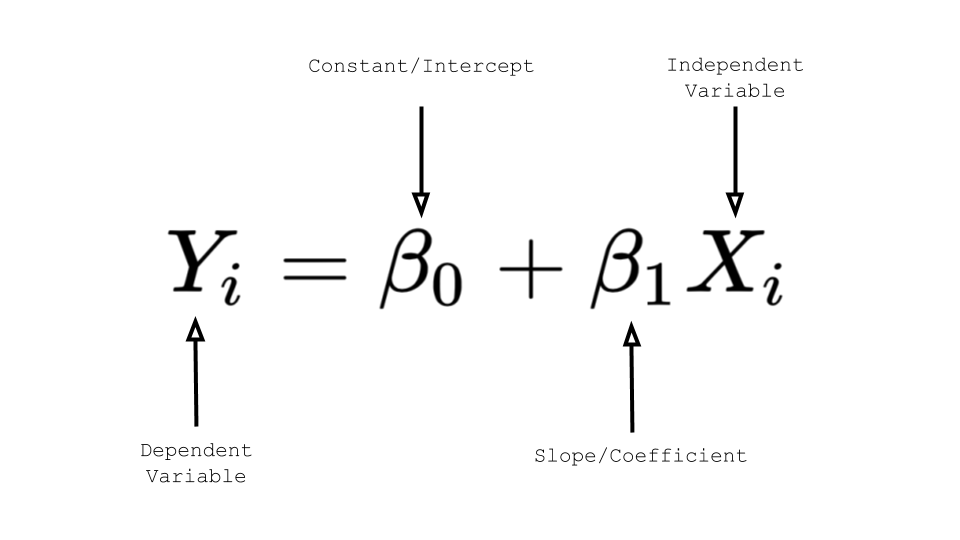
Unlike in pure mathematics, in machine learning, the relationship denoted by the linear equation is an approximation. That’s why we refer to the slope and the intercept as parameters and we must estimate these parameters for our linear regression. We even use a different notation in which the intercept constant is written first and the variables are greek symbols:

Simple Linear Regression in Python (From Scratch) | by Aidan Wilson | Towards Data Science

Even though the notation is different, it’s the exact same equation of a line y=mx+b. It is important to know this notation though because it may come up in other linear regression material.

But how do we know where to make the linear regression line when the points are not straight in a row? There are a whole bunch of lines that can be drawn through scattered data points. How do we know which one is the “best” line?

There will usually be a gap between the actual value and the line. In other words, there is a difference between the actual data point and the point on the line (fitted value/predicted value). These gaps are called residuals. The residuals can tell us something about how “good” of an estimate our line is making.

Look at the size of the residuals and choose the line with the smallest residuals. Now, we have a clear method for the hazy goal of representing the relationship as a straight line. The objective of the linear regression algorithm is to calculate the line that minimizes these residuals.

For each possible line (slope and intercept pair) for a set of data:

Calculate the residuals
Square them to prevent negatives
Add the sum of the squared residuals

Then, choose the slope and intercept pair that minimizes the sum of the squared residuals, also known as Residual Sum of Squares.

Linear regression models can also be used to estimate the value of the dependent variable for a given independent variable value. Using the classic linear equation, you would simply substitute the value you want to test for x in y = mx + b; y would be the model’s prediction for the target for your given feature value x.

Linear Regression in Python

Now that we’ve discussed the theory around Linear Regression, let’s take a look at an example.

Let’s say we are running an ice cream shop. We have collected some data for daily ice cream sales and the temperature on those days. The data is stored in a file called temp_revenue_data.csv. We want to see how strong the correlation between the temperature and our ice cream sales is.

import pandas
from pandas import DataFrame 

data = pandas.read_csv('temp_revenue_data.csv')

X = DataFrame(data, columns=['daily_temperature'])
y = DataFrame(data, columns=['ice_cream_sales'])

First, import Linear Regression from the scikitlearn module (a machine learning module in Python). This will allow us to run linear regression models in just a few lines of code.

from sklearn.linear_model import LinearRegression

Next, create a LinearRegression() object and store it in a variable.

regression = LinearRegression()

Now that we’ve created our object we can tell it to do something:

The fit method runs the actual regression. It takes in two parameters, both of type DataFrame. The feature data is the first parameter and the target data is the second. We are using the X and y DataFrames defined above.

regression.fit(X, y)

The slope and intercept that were calculated by the regression are available in the following properties of the regression object: coef_ and intercept_. The trailing underline is necessary.

# Slope Coefficient
regression.coef_

# Intercept
regression.intercept_

How can we quantify how “good” our model is? We need some kind of measure or statistic. One measure that we can use is called R², also known as the goodness of fit.

regression.score(X, y)
output: 0.5496...

The above output number (in percentage) is the amount of variation in ice cream sales that is explained by the daily temperature.

Note: The model is very simplistic and should be taken with a grain of salt. It especially does not do well on the extremes.