LeetCode #125: Valid Palindrome (Solution in Python & Explanation)

In this article, I will be explaining how to solve the Valid Palindrome problem on LeetCode. This is an Easy-level problem.

The Problem

A phrase is a palindrome if, after converting all uppercase letters into lowercase letters and removing all non-alphanumeric characters, it reads the same forward and backward. Alphanumeric characters include letters and numbers.

Given a string s, return true if it is a palindrome, or false otherwise.

Example 1:

Input: s = "A man, a plan, a canal: Panama"
Output: true
Explanation: "amanaplanacanalpanama" is a palindrome.

Example 2:

Input: s = "race a car"
Output: false
Explanation: "raceacar" is not a palindrome.

Example 3:

Input: s = " "
Output: true
Explanation: s is an empty string "" after removing non-alphanumeric characters.
Since an empty string reads the same forward and backward, it is a palindrome.

Solution

Alphanumeric characters are the lowercase letters a-z, capital letters A-Z, and integers 0-9.

So, to solve this, we first want to remove all non-alphanumeric characters, including spaces, punctuation, etc., from the input string. Then, we need to check the new string to see if it’s a palindrome. We have two ways we can do this.

Solution #1

For this solution, we create a new string which contains all of the alphanumeric characters from the input string (lowercased). Then, we compare this new string to its reversed version. If they are the same, the function returns true. If not, it returns false.

In order to create the new string, we loop through the characters in the original input string and, if the character is alphanumeric, we append it to the new string.

Finally, we can check if the string (without any special characters or spaces) is a palindrome by using a boolean expression to equate it to its reverse. We can get the reverse of a string by using str[::-1]

def isPalindrome(self, s: str) -> bool:
    newStr = ""
    
    for char in s:
        if char.isalnum():
            newStr += c.lower()
    return newStr == newStr[::-1]

This solution has a time complexity of O(n) because we have to loop through the string to remove non-alphanumeric characters. It also has a space complexity of O(n) because we are creating another string, which could be at most the size of the input string.

Solution #2

For this solution, we will create pointers to the beginning and end of the array which will make sure that the two sides have the same characters in the same order.

First, create two pointers— one which points to the beginning of the string and the other which points to the end. The two pointers will move inwards, checking each character until the reach the middle or overlap with each other.

As the pointers loop through the characters, they will skip any characters that are not alphanumeric. To do this, we use while loops that will continue to run until the character at the left/right index is alphanumeric. We also add a check to make sure that the left/right index is in bounds by checking left < right / right > left

We must make sure to compare the lowercase versions of the characters to each other. If any character at the left pointer does not match the corresponding character at the right pointer, then we know that it’s not a palindrome and can return False. If the entire loop finishes then that must mean the string is a palindrome and we can return True.

def isPalindrome(self, s: str) -> bool:
    left, right = 0, len(s) - 1 
 
    while left < right:
        while left < right and not s[left].isalnum():
            left +=1
        while right > left and not s[right].isalnum():
            right -= 1
        if s[left].lower() != s[right].lower():
            return False 
        left, right = left + 1, right - 1
    return True

The time complexity for this solution is O(n) because you are still looping through the entire string. The space complexity is O(1) because you are not making a new string.

LeetCode #242: Valid Anagrams (Solution in Python & Explanation)

The Problem

Given two strings s and t, return true if t is an anagram of s, and false otherwise.

An Anagram is a word or phrase formed by rearranging the letters of a different word or phrase, typically using all the original letters exactly once.

Example 1:

Input: s = "anagram", t = "nagaram"
Output: true

Example 2:

Input: s = "rat", t = "car"
Output: false

Solution

We know that the two strings are anagrams if:

  1. They have the same length
  2. They have the same characters and the same quantity of each character

So, if we can verify that the strings pass these two criteria, we can verify that they are valid anagrams.

We can check if they are the same length by simply using len:

len(s) == len(t)   # boolean expression

But how can we check if they have the same characters and the same quantity of each character? We can use hash maps. For each string, we can create a hash map that includes every unique character in the string and its frequency in the string.

For example, this would be the hash map of the string s, which has a value of "anagram":

s = "anagram"
countS = {"a": 3, "n": 1, "g": 1, "m": 1}

Once, we have created the hash maps, we can check if they are equivalent by using a boolean expression:

countS == countT

So, let’s put it all together. These are all the steps we have to take:

  1. We check if the strings are not the same length. If they’re not, we can immediately return False without doing any other code.
  2. We create empty hash maps for the two strings s and t.
  3. We loop through each character in s and t and add them to the hash maps. If the character does not exist in the hash map, a new key for the character is added and the value is initialized to 0 (then we add 1). If a key for the character does exist in the hash map, we add 1 to the value.
  4. We check if the two hash maps are equivalent. If they are, we return True. If they are not, we return False.

This is the final code.

   def isAnagram(self, s: str, t: str) -> bool:
        # Step 1: check if same length
        if len(s) != len(t):
            return False
        
        # Step 2: create hash maps
        countS = {}
        countT = {}
        
        # Step 3: loop through characters to add to hash map
        for i in range(len(s)):
            countS[s[i]] = 1 + countS.get(s[i], 0)
            countT[t[i]] = 1 + countT.get(t[i], 0)
        
        # Step 4: check if hash maps are equivalent  
        if (countS == countT): 
            return True
        else: 
            return False

This solution has a time complexity of O(s + t) or simply O(n) because we have to iterate through each of the strings. The space complexity is also O(s + t) because we are building hash maps that are the sizes of arrays s and t.

There is another solution that is much more simple, but less efficient. We can sort both of the strings and see if the sorted versions are equivalent. This works because, if they are anagrams, then they will have the same sorted value.

def isAnagram(self, s: str, t: str) -> bool:
    return sorted(s) == sorted(t)

A good sorting algorithm can sort an array of characters in O(n * log(n)) time. The space complexity could be either O(1) or O(n)

Overlapping Histograms with Matplotlib Library in Python

In this tutorial, you will learn how to plot overlapping histograms on the same graph. This is helpful when you want to show a comparison between two sets of data.

Step 1: Import the matplotlib library and matplotlib.pyplot interface

import pandas as pd

import matplotlib
%matplotlib inline
import matplotlib.pyplot as plt

Step 2: Load the dataset

baby_df = pd.read_csv('baby.csv')
baby_df.head(5)

Step 3: Plot overlapping histograms

# Split the dataframe by column value
smoker_df = baby_df.loc[baby_df['Maternal Smoker'] == True]
nonsmoker_df = baby_df.loc[baby_df['Maternal Smoker'] == False]

# Generate histogram plot
plt.hist(smoker_df["bmi"], 
         label='Maternal Smokers BMI')
  
plt.hist(nonsmoker_df['bmi'], 
         label='Maternal Non-smokers BMI')
  
plt.legend(loc='upper right')
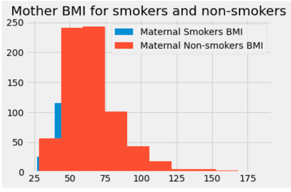
plt.title('Mother BMI for smokers and non-smokers')
plt.show()

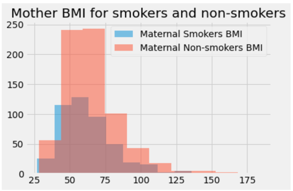
We’ve generated overlapping histograms! But, in this graph, it’s hard to see the blue histogram. We can give the histograms an opacity value less than 1.0 so that they become translucent, or see-through. This will allow us to see both of them.

Set alpha values

The only difference is adding the optional alpha parameter to the hist method. The alpha value can be any decimal between 0 and 1. Each plot can have a unique alpha value.

# Generate histogram plot
plt.hist(smoker_df["bmi"], 
         alpha=0.5,
         label='Maternal Smokers BMI')
  
plt.hist(nonsmoker_df['bmi'], 
         alpha=0.5
         label='Maternal Non-smokers BMI')

You can also have more than 2 overlapping plots. In this case, it can be helpful to manually set the color for each histogram. We can do this by adding the color parameter to each hist call:

plt.hist(dataset['value'], 
         alpha=0.5, 
         label='val 1',
         color='red') # customized color parameter
  
plt.hist(dataset['value2'], 
         alpha=0.5,
         label='val 2',
         color='green')
  
plt.hist(dataset['value3'], 
         alpha=0.5,
         label='val3',
         color='yellow')

Calculate Derivative Functions in Python

In machine learning, derivatives are used for solving optimization problems. Optimization algorithms such as gradient descent use derivatives to decide whether to increase or decrease the weights in order to get closer and closer to the maximum or minimum of a function. This post covers how these functions are used in Python.

Symbolic differentiation manipulates a given equation, using various rules, to produce the derivative of that equation. If you know the equation that you want to take the derivative of, you can do symbolic differentiation in Python. Let’s use this equation as an example:

f(x) = 2x2+5

Import SymPy

In order to do symbolic differentiation, we’ll need a library called SymPy. SymPy is a Python library for symbolic mathematics. It aims to be a full-featured computer algebra system (CAS). First, import SymPy:

from sympy import *

Make a symbol

Variables are not defined automatically in SymPy. They need to be defined explicitly using symbols. symbols takes a string of variable names separated by spaces or commas, and creates Symbols out of them. Symbol is basically just the SymPy term for a variable.

Our example function f(x) = 2x2+5 has one variable x, so let’s create a variable for it:

x = symbols('x')

If the equation you’re working with has multiple variables, you can define them all in one line:

x, y, z = symbols('x y z')

Symbols can be used to create symbolic expressions in Python code.

>>> x**2 + y         
x2+y
>>> x**2 + sin(y)   
x2+sin(y)

Write symbolic expression

So, using our Symbol x that we just defined, let’s create a symbolic expression in Python for our example function f(x) = 2x2+5:

f = 2*x**2+5

Take the derivative

Now, we’ll finally take the derivative of the function. To compute derivates, use the diff function. The first parameter of the diff function should be the function you want to take the derivative of. The second parameter should be the variable you are taking the derivative with respect to.

x = symbols('x')
f = 2*x**2+5

df = diff(f, x)

The output for the f and df should look like this:

>>> f
2*x**2+5
>>> df
4*x

You can take the nth derivative by adding an optional third argument, the number of times you want to differentiate. For example, taking the 3rd derivative:

d3fd3x = diff(f, x, 3)

Substituting values into expressions

So we are able to make symbolic functions and compute their derivatives, but how do we use these functions? We need to be able to plug a value into these equations and get a solution.

We can substitute values into symbolic equations using the subs method. The subs method replaces all instances of a variable with a given value. subs returns a new expression; it doesn’t modify the original one. Here we substitute 4 for the variable x in df:

>>> df.subs(x, 4)
16

To evaluate a numerical expression into a floating point number, use evalf.

>>> df.subs(x, 4).evalf()
16.0

To perform multiple substitutions at once, pass a list of (old, new) pairs to subs. Here’s an example:

>>> expr = x**3 + 4*x*y - z
>>> expr.subs([(x, 2), (y, 4), (z, 0)])
40

The lambdify function

If you are only evaluating an expression at one or two points, subs and evalf work well. But if you intend to evaluate an expression at many points, you should convert your SymPy expression to a numerical expression, which gives you more options for evaluating expressions, including using other libraries like NumPy and SciPy.

The easiest way to convert a symbolic expression into a numerical expression is to use the lambdify function.

The lambdify function takes in a Symbol and the function you are converting. It returns the converted function. Once the function is converted to numeric, you can Let’s convert the function and derivative function from our example.

>>> f = lambdify(x, f)
>>> df = lambdify(x, df)
>>> f(3)
23
>>> df(3)
12

Here’s an example of using lambdify with NumPy:

>>> import numpy
>>> test_numbers = numpy.arange(10)   
>>> expr = sin(x)
>>> f(test_numbers)
[ 0.          0.84147098  0.90929743  0.14112001 -0.7568025  -0.95892427  -0.2794155   0.6569866   0.98935825  0.41211849]

The application of these functions in a data science solution will be covered in another post.

Introduction to Gradient Descent with Python

In this article, I’m going to talk about a popular optimization algorithm in machine learning: gradient descent. I’ll explain what gradient descent is, how it works, and then we’ll write the gradient descent algorithm from scratch in Python. This article assumes you are familiar with derivatives in Calculus.

What is Gradient Descent?

Gradient descent is an optimization algorithm for finding the minimum of a function. The algorithm does this by checking the steepness of the slope along the graph of a line and using that to slowly move towards the lowest point, which presumably has a slope of 0. Write an algorithm to find the lowest cost.

You can think of gradient descent as akin to a blind-folded hiker on top of a mountain trying to get to the bottom. The hiker must feel the incline, or the slope, of the mountain in order to get an idea of where she is going. If the slope is steep, the hiker is closer to the peak and can take bigger steps. If the slope is less steep, the hiker is closer to the bottom and takes smaller steps. If the hiker feels flat ground (a zero slope), she can assume she’s reached the bottom, or minimum.

So given a function with a convex graph, the gradient descent algorithm attempts to find the minimum of the function by using the derivative to check the steepness of points along the line and slowly move towards a slope of zero. After all, “gradient” is just another word for slope.

Implement Gradient Descent in Python

Before we start, import the SymPy library and create a “symbol” called x. We’ll be needing these lines later when we are working with math functions and derivatives.

from sympy import *
x = Symbol('x')

We create our gradient_descent function and give it two parameters: cost_fn, starting_point and learning_rate. The cost_fn is the math function that we want to find the minimum of. The initial_guess parameter is the integer that is our first guess for the x-value of the minimum of the function. We will update this variable to be our new guess after each learning iteration. The last parameter is the learning rate.

def gradient_descent(cost_fn, initial_guess, learning_rate):
    df = cost_fn.diff(x)
    df = lambdify(x, df)

    new_x = initial_guess

    for n in range(100):
        # Step 1: Predict (Make a guess)
        previous_x = new_x

        # Step 2: Calculate the error
        gradient = df(previous_x)

        # Step 3: Learn (Make adjustments)
        new_x = previous_x - learning_rate * gradient

Inside the function, we first get the derivative of the cost function that was inputted as a parameter using the diff function of the SymPy library. We store the derivative in the df variable. Then, we use the lambdify function because it allows us to plug our predictions into the derivative function. Read my article on calculating derivatives in Python for more info on this.

In the for loop, our gradient descent function is following the 3-step algorithm that is used to train many machine learning tools:

  1. Predict (Make a guess)
  2. Calculate the error
  3. Learn (Make adjustments)

You can learn more about this process in this article on how machines “learn.”

In the for loop, the first step is to make an arbitrary guess for the x-value of the minimum of the function. We do this by setting previous_x to new_x, which is the user’s initial guess. previous_value will help us keep track of the preceding prediction value as we make new guesses.

Next, we calculate the error or, in other words, we see how far our current guess is from the minimum of the function. We do this by calculating the derivative of the function at the point we guessed, which will give us the slope at that point. If the slope is large, the guess is far from the minimum. But if the slope is close to 0, the guess is getting closer to the minimum.

Next, we “learn” from the error. In the previous step, we calculated the slope at the x-value that we guessed. We multiply that slope by the learning_rate and subtract that from the current guess value stored in previous_x. Then, we store this new guess value back into new_x.

Then, we run these steps over and over in our for loop until the loop is over.

Before we run our gradient descent function, let’s add some print statements at the end so we can see the values of at the minimum of the function.

print('Minimum occurs at x-value:', min_x)
print('Slope at the minimum is: ', df(min_x))

Now, let’s run our gradient descent function and see what type of output we get with an example. In this example, the cost function is f(x) = x2. The initial guess for x is 3 and the learning rate is 0.1

my_fn = x**2
gradient_descent(my_fn, 3, 0.1)

Currently, we are running the learning loop an arbitrary amount of times. In this example, the loop runs 100 times. But maybe we don’t need to run the loop this many times. Oftentimes you already know ahead of time how precise a calculate you need. You can tell the loop to stop running once a certain level of precision is met. There are many ways you can implement this, but I’ll show you using that for loop we already have.

precision = 0.0001

for n in range(100):
    previous_x = new_x
    gradient = df(previous_x)
    new_x = previous_x - learning_rate * gradient
    
    step_size = abs(new_x - previous_x) 
    
    if step_size < precision:
        break

First, we define a precision value that the gradient descent algorithm should be within. You can also make this a parameter to the function if you choose.

Inside the loop, we create a new variable called step_size which is the distance between previous_x and new_x, which is the new guess that was just calculated in the “learning” step. We take the absolute value of this difference in case it’s negative.

If the step_size is less than the precision we specified, the loop will finish, even if it hasn’t reached 100 iterations yet.

Instead of solving a cost function analytically, the gradient descent algorithm converges on the minimum of a function by brute force. Like a blind-folded hiker, the algorithm goes down the valley (the cost function), following the slope of the graph until it reaches the minimum point.