Calculate Derivative Functions in Python

In machine learning, derivatives are used for solving optimization problems. Optimization algorithms such as gradient descent use derivatives to decide whether to increase or decrease the weights in order to get closer and closer to the maximum or minimum of a function. This post covers how these functions are used in Python.

Symbolic differentiation manipulates a given equation, using various rules, to produce the derivative of that equation. If you know the equation that you want to take the derivative of, you can do symbolic differentiation in Python. Let’s use this equation as an example:

f(x) = 2x2+5

Import SymPy

In order to do symbolic differentiation, we’ll need a library called SymPy. SymPy is a Python library for symbolic mathematics. It aims to be a full-featured computer algebra system (CAS). First, import SymPy:

from sympy import *

Make a symbol

Variables are not defined automatically in SymPy. They need to be defined explicitly using symbols. symbols takes a string of variable names separated by spaces or commas, and creates Symbols out of them. Symbol is basically just the SymPy term for a variable.

Our example function f(x) = 2x2+5 has one variable x, so let’s create a variable for it:

x = symbols('x')

If the equation you’re working with has multiple variables, you can define them all in one line:

x, y, z = symbols('x y z')

Symbols can be used to create symbolic expressions in Python code.

>>> x**2 + y         
x2+y
>>> x**2 + sin(y)   
x2+sin(y)

Write symbolic expression

So, using our Symbol x that we just defined, let’s create a symbolic expression in Python for our example function f(x) = 2x2+5:

f = 2*x**2+5

Take the derivative

Now, we’ll finally take the derivative of the function. To compute derivates, use the diff function. The first parameter of the diff function should be the function you want to take the derivative of. The second parameter should be the variable you are taking the derivative with respect to.

x = symbols('x')
f = 2*x**2+5

df = diff(f, x)

The output for the f and df should look like this:

>>> f
2*x**2+5
>>> df
4*x

You can take the nth derivative by adding an optional third argument, the number of times you want to differentiate. For example, taking the 3rd derivative:

d3fd3x = diff(f, x, 3)

Substituting values into expressions

So we are able to make symbolic functions and compute their derivatives, but how do we use these functions? We need to be able to plug a value into these equations and get a solution.

We can substitute values into symbolic equations using the subs method. The subs method replaces all instances of a variable with a given value. subs returns a new expression; it doesn’t modify the original one. Here we substitute 4 for the variable x in df:

>>> df.subs(x, 4)
16

To evaluate a numerical expression into a floating point number, use evalf.

>>> df.subs(x, 4).evalf()
16.0

To perform multiple substitutions at once, pass a list of (old, new) pairs to subs. Here’s an example:

>>> expr = x**3 + 4*x*y - z
>>> expr.subs([(x, 2), (y, 4), (z, 0)])
40

The lambdify function

If you are only evaluating an expression at one or two points, subs and evalf work well. But if you intend to evaluate an expression at many points, you should convert your SymPy expression to a numerical expression, which gives you more options for evaluating expressions, including using other libraries like NumPy and SciPy.

The easiest way to convert a symbolic expression into a numerical expression is to use the lambdify function.

The lambdify function takes in a Symbol and the function you are converting. It returns the converted function. Once the function is converted to numeric, you can Let’s convert the function and derivative function from our example.

>>> f = lambdify(x, f)
>>> df = lambdify(x, df)
>>> f(3)
23
>>> df(3)
12

Here’s an example of using lambdify with NumPy:

>>> import numpy
>>> test_numbers = numpy.arange(10)   
>>> expr = sin(x)
>>> f(test_numbers)
[ 0.          0.84147098  0.90929743  0.14112001 -0.7568025  -0.95892427  -0.2794155   0.6569866   0.98935825  0.41211849]

The application of these functions in a data science solution will be covered in another post.

Introduction to Gradient Descent with Python

In this article, I’m going to talk about a popular optimization algorithm in machine learning: gradient descent. I’ll explain what gradient descent is, how it works, and then we’ll write the gradient descent algorithm from scratch in Python. This article assumes you are familiar with derivatives in Calculus.

What is Gradient Descent?

Gradient descent is an optimization algorithm for finding the minimum of a function. The algorithm does this by checking the steepness of the slope along the graph of a line and using that to slowly move towards the lowest point, which presumably has a slope of 0. Write an algorithm to find the lowest cost.

You can think of gradient descent as akin to a blind-folded hiker on top of a mountain trying to get to the bottom. The hiker must feel the incline, or the slope, of the mountain in order to get an idea of where she is going. If the slope is steep, the hiker is closer to the peak and can take bigger steps. If the slope is less steep, the hiker is closer to the bottom and takes smaller steps. If the hiker feels flat ground (a zero slope), she can assume she’s reached the bottom, or minimum.

So given a function with a convex graph, the gradient descent algorithm attempts to find the minimum of the function by using the derivative to check the steepness of points along the line and slowly move towards a slope of zero. After all, “gradient” is just another word for slope.

Implement Gradient Descent in Python

Before we start, import the SymPy library and create a “symbol” called x. We’ll be needing these lines later when we are working with math functions and derivatives.

from sympy import *
x = Symbol('x')

We create our gradient_descent function and give it two parameters: cost_fn, starting_point and learning_rate. The cost_fn is the math function that we want to find the minimum of. The initial_guess parameter is the integer that is our first guess for the x-value of the minimum of the function. We will update this variable to be our new guess after each learning iteration. The last parameter is the learning rate.

def gradient_descent(cost_fn, initial_guess, learning_rate):
    df = cost_fn.diff(x)
    df = lambdify(x, df)

    new_x = initial_guess

    for n in range(100):
        # Step 1: Predict (Make a guess)
        previous_x = new_x

        # Step 2: Calculate the error
        gradient = df(previous_x)

        # Step 3: Learn (Make adjustments)
        new_x = previous_x - learning_rate * gradient

Inside the function, we first get the derivative of the cost function that was inputted as a parameter using the diff function of the SymPy library. We store the derivative in the df variable. Then, we use the lambdify function because it allows us to plug our predictions into the derivative function. Read my article on calculating derivatives in Python for more info on this.

In the for loop, our gradient descent function is following the 3-step algorithm that is used to train many machine learning tools:

  1. Predict (Make a guess)
  2. Calculate the error
  3. Learn (Make adjustments)

You can learn more about this process in this article on how machines “learn.”

In the for loop, the first step is to make an arbitrary guess for the x-value of the minimum of the function. We do this by setting previous_x to new_x, which is the user’s initial guess. previous_value will help us keep track of the preceding prediction value as we make new guesses.

Next, we calculate the error or, in other words, we see how far our current guess is from the minimum of the function. We do this by calculating the derivative of the function at the point we guessed, which will give us the slope at that point. If the slope is large, the guess is far from the minimum. But if the slope is close to 0, the guess is getting closer to the minimum.

Next, we “learn” from the error. In the previous step, we calculated the slope at the x-value that we guessed. We multiply that slope by the learning_rate and subtract that from the current guess value stored in previous_x. Then, we store this new guess value back into new_x.

Then, we run these steps over and over in our for loop until the loop is over.

Before we run our gradient descent function, let’s add some print statements at the end so we can see the values of at the minimum of the function.

print('Minimum occurs at x-value:', min_x)
print('Slope at the minimum is: ', df(min_x))

Now, let’s run our gradient descent function and see what type of output we get with an example. In this example, the cost function is f(x) = x2. The initial guess for x is 3 and the learning rate is 0.1

my_fn = x**2
gradient_descent(my_fn, 3, 0.1)

Currently, we are running the learning loop an arbitrary amount of times. In this example, the loop runs 100 times. But maybe we don’t need to run the loop this many times. Oftentimes you already know ahead of time how precise a calculate you need. You can tell the loop to stop running once a certain level of precision is met. There are many ways you can implement this, but I’ll show you using that for loop we already have.

precision = 0.0001

for n in range(100):
    previous_x = new_x
    gradient = df(previous_x)
    new_x = previous_x - learning_rate * gradient
    
    step_size = abs(new_x - previous_x) 
    
    if step_size < precision:
        break

First, we define a precision value that the gradient descent algorithm should be within. You can also make this a parameter to the function if you choose.

Inside the loop, we create a new variable called step_size which is the distance between previous_x and new_x, which is the new guess that was just calculated in the “learning” step. We take the absolute value of this difference in case it’s negative.

If the step_size is less than the precision we specified, the loop will finish, even if it hasn’t reached 100 iterations yet.

Instead of solving a cost function analytically, the gradient descent algorithm converges on the minimum of a function by brute force. Like a blind-folded hiker, the algorithm goes down the valley (the cost function), following the slope of the graph until it reaches the minimum point.

Introduction to Linear Regression

In this article, I will define what linear regression is in machine learning, delve into linear regression theory, and go through a real-world example of using linear regression in Python.

What is Linear Regression?

Linear regression is a machine learning algorithm used to measure the relationship between two variables. The algorithm attempts to model the relationship between the two variables by fitting a linear equation to the data.

In machine learning, these two variables are called the feature and the target. The feature, or independent variable, is the variable that the data scientist uses to make predictions. The target, or dependent variable, is the variable that the data scientist is trying to predict.

Before attempting to fit a linear regression to a set of data, you should first assess if the data appears to have a relationship. You can visually estimate the relationship between the feature and the target by plotting them on a scatterplot.

If you plot the data and suspect that there is a relationship between the variables, you can verify the nature of the association using linear regression.

Linear Regression Theory

Linear regression will try to represent the relationship between the feature and target as a straight line.

Do you remember the equation for a straight line that you learned in grade school?

y = mx + b, where m is the slope (the number describing the steepness of the line) and b is the y-intercept (the point at which the line crosses the vertical axis)

Equation of a Straight Line

Equations describing linear regression models follow this same format.

The slope m tells you how strong the relationship between x and y is. The slope tells us how much y will go up or down for a given increase or decrease in x, or, in this case, how much the target will change for a given change in the feature.

In theory, a slope of 0 would mean there is no relationship at all between the data. The weaker the relationship is, the closer the slope is to 0. But if there is a strong relationship, the slope will be a larger positive or negative number. The stronger the relationship is, the steeper the slope is.

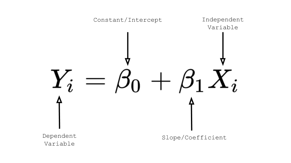
Unlike in pure mathematics, in machine learning, the relationship denoted by the linear equation is an approximation. That’s why we refer to the slope and the intercept as parameters and we must estimate these parameters for our linear regression. We even use a different notation in which the intercept constant is written first and the variables are greek symbols:

Simple Linear Regression in Python (From Scratch) | by Aidan Wilson |  Towards Data Science

Even though the notation is different, it’s the exact same equation of a line y=mx+b. It is important to know this notation though because it may come up in other linear regression material.

But how do we know where to make the linear regression line when the points are not straight in a row? There are a whole bunch of lines that can be drawn through scattered data points. How do we know which one is the “best” line?

There will usually be a gap between the actual value and the line. In other words, there is a difference between the actual data point and the point on the line (fitted value/predicted value). These gaps are called residuals. The residuals can tell us something about how “good” of an estimate our line is making.

Look at the size of the residuals and choose the line with the smallest residuals. Now, we have a clear method for the hazy goal of representing the relationship as a straight line. The objective of the linear regression algorithm is to calculate the line that minimizes these residuals.

For each possible line (slope and intercept pair) for a set of data:

  1. Calculate the residuals
  2. Square them to prevent negatives
  3. Add the sum of the squared residuals

Then, choose the slope and intercept pair that minimizes the sum of the squared residuals, also known as Residual Sum of Squares.

Linear regression models can also be used to estimate the value of the dependent variable for a given independent variable value. Using the classic linear equation, you would simply substitute the value you want to test for x in y = mx + b; y would be the model’s prediction for the target for your given feature value x.

Linear Regression in Python

Now that we’ve discussed the theory around Linear Regression, let’s take a look at an example.

Let’s say we are running an ice cream shop. We have collected some data for daily ice cream sales and the temperature on those days. The data is stored in a file called temp_revenue_data.csv. We want to see how strong the correlation between the temperature and our ice cream sales is.

import pandas
from pandas import DataFrame 

data = pandas.read_csv('temp_revenue_data.csv')

X = DataFrame(data, columns=['daily_temperature'])
y = DataFrame(data, columns=['ice_cream_sales'])

First, import Linear Regression from the scikitlearn module (a machine learning module in Python). This will allow us to run linear regression models in just a few lines of code.

from sklearn.linear_model import LinearRegression

Next, create a LinearRegression() object and store it in a variable.

regression = LinearRegression()

Now that we’ve created our object we can tell it to do something:

The fit method runs the actual regression. It takes in two parameters, both of type DataFrame. The feature data is the first parameter and the target data is the second. We are using the X and y DataFrames defined above.

regression.fit(X, y)     

The slope and intercept that were calculated by the regression are available in the following properties of the regression object: coef_ and intercept_. The trailing underline is necessary.

# Slope Coefficient
regression.coef_

# Intercept
regression.intercept_

How can we quantify how “good” our model is? We need some kind of measure or statistic. One measure that we can use is called R2, also known as the goodness of fit.

regression.score(X, y)
output: 0.5496...

The above output number (in percentage) is the amount of variation in ice cream sales that is explained by the daily temperature.

Note: The model is very simplistic and should be taken with a grain of salt. It especially does not do well on the extremes.

How to Set Up a New Django Project

Django is a high-level Python web framework that enables rapid development of secure and maintainable websites. It is one of the most popular Python backend development frameworks. It is known for its security, simplicity, and reliability. It is without a doubt one of the best frameworks to learn.

Note: You must have Python 3 or later installed on your computer to complete this tutorial.

Create a new empty project. The first thing we need to do is install Django in our new project. You might be tempted to do it using the command pip install django, but I would advise against this because it installs the Django package on your global system rather than just in this specific project.

Instead, you should use a tool called pipenv, which allows you to set up a virtual environment for each Python project that you create on your system. Install it globally by running this command:

pip install pipenv

With pipenv installed, run this command in your project folder to create a virtual environment.

pipenv shell

Any packages we install, including Django, will be installed into this virtual environment rather than on our global system. This command will also generate a Pipfile in your project directory. This Pipfile will list any packages that you install in the virtual environment.

Run this command to install Django in the virtual environment

pipenv install django

In Django, a project is basically the overall website/application. Then, you have the concept of apps; there are usually multiple apps in each project.

Run this command to create a new project (put your project’s name in place of project-name):

django-admin startproject project-name 
cd project-name 

Inside your new project folder, you should see a second folder with the same project name and a manage.py file. You rarely change any of the code in the manage.py file, but you will use this file all the time. We use this file to run the server, create migrations, and carry out many other commands.

Once inside the project folder we just created, run this command to run the server on http: 127.0.0.1:8000 (port 8000):

python manage.py runserver
# ctrl+c to stop

To run the server on a different port

python manage.py runserver 8081

You will probably get the below error. The cause of the error is that there are migrations ready to create the default, necessary database tables that Django uses that have not been applied.

To apply them, we run this command:

python manage.py migrate

Now, your server should be up and running with no errors. If you type localhost:8000 (or whichever port your project is running on) in your browser, you should see this default Django page.

You’ve officially created your first Django project. The next step is to start adding apps to your project. Stay tuned for a tutorial on that.

Python Tutorial: Web Scraping with BeautifulSoup and Requests

Web scraping is the process of automatically extracting data from a website.

You will need an understanding of basic HTML page structure in order to grasp this tutorial. Web scraping with BeautifulSoup to get data/text from a page is done by referencing specific HTML semantic tags, classes, and ids on that page and getting the data from within them. You will better understand what I mean as we continue.

BeautifulSoup is the Python package we are going to use to do the web scraping. Requests is a package that allows you to send HTTP/1.1 requests extremely easily.

In this tutorial, we are going to be parsing the information from the daily forecast element on the Orlando, FL weather page on weather.com (this is the link). We will transfer the information to a structured, table format using Pandas.

The picture below shows the div element which holds the daily forecast information for the week. When you view this tutorial, the numbers will probably not be the same but, other than that, you should see something that looks like this. This is the element we are going to be scraping.

In Terminal, create a new folder with mkdir, cd into the folder, and create a .py file. I will call mine scraper.py. This file will contain the code for the scraper.

In the next lines, we are installing some necessary dependencies using pip, the Python package manager, into our project folder.

mkdir project-folder
cd project-folder
touch scraper.py
pip install beautifulsoup4
pip install requests
pip install pandas

Open up the scraper.py file in a Code Editor.

First, we will add the import statements to our file for the packages we just installed using pip:

from bs4 import BeautifulSoup
import requests

Ok, let’s start writing the code. First, write the following line:

page = requests.get('https://weather.com/weather/today/l/9ca5fcd4263a24d4d3aaea0c6ab0aea6bea876cfce908ee624588a8f269f6fa1')

This line uses the request package to get the HTML page of the URL in quotes. In this case, we are using a page on the site.

Next, write this line:

soup = BeautifulSoup(page.content, 'html.parser')

This line initializes BeautifulSoup in our project. Now, we can use the soup variable to access the functions within the BeautifulSoup package. The first parameter in the statement is what you want to scrape (in this case, the content of the page we got earlier) and the second parameter just tells BeautifulSoup that it will be parsing HTML.

Now, if you are using Google Chrome, you can Inspect the page and find the id of the div element which holds the data you want to scrape.

As you can see from the above image, I found that the div containing the Daily Forecast information had an id of “WxuDailyWeatherCard-main-bb1a17e7-dc20-421a-b1b8-c117308c6626”

After getting the id of the div element which holds the data we want, we are defining a reference to the div element with the following line:

week = soup.find(id='WxuDailyWeatherCard-main-bb1a17e7-dc20-421a-b1b8-c117308c6626')

Now we can use the variable week to reference the Daily Forecast div.

Using Inspect again, I found that the actual content within the div element is stored in a elements with a class of “Column–innerWrapper–3K14X”.

We can get access to all 5 (one for each day of the week) of these a tag items using the find_all function.

items = week.find_all(class_='Column--innerWrapper--3K14X')

Now, we can get access to the data within the items array. We will make an array of the dates within the items array using this line:

date = [item.find('h3', class_='Column--label--L3RrD').get_text() for item in items]

Using the same process as before, I found that all the dates were stored in a h3 with a class of ‘Column–label–L3RrD’. The above line creates an array of dates by running the find() method on every item within the items array.

Now, we can do this for the temperature and chance of rain data stored in the items array.

temp = [item.find(class_='Column--temp--2v_go').get_text() for item in items]

chanceOfRain = [item.find(class_='Column--precip--2H5Iw').get_text() for item in items]

Now, you can access the date, temperature, and chance of rain data with the variables we just created!

Pandas Addition

As an extra, you can put the weather data we just scraped into a simple Panda’s data frame so that it looks better.

First, install the Pandas package and import Pandas at the top of your scraper.py file.

import pandas as pd

Under the data definitions, write this line. This line creates a data frame in the variable weather_info with the data.

weather_info = pd.DataFrame({
    'Date': date,
    'Temp': temp,
    'Chance Of Rain': chanceOfRain
})

You can print the weather info to see your data outputted in a table format

print(weather_info)

And that’s it! You’re done. Here is the full code:

Here is the expected output– a Pandas data frame. You can do some research and see how to make it look better:

How to Execute a Python Script in a Node.js Project

This tutorial assumes that you’ve already set up a basic Node.js project with Express. I have other tutorials explaining how to do this if you don’t know how.

First, create a new python file in your Node project directory. I will call mine hello.py. In hello.py, I will write a simple Python print statement to test.

print("Hello world")

In my main JavaScript file, I’m going to add the bolded line:

const express = require('express');
const { spawn } = require('child_process');

const app = express();

app.get('/', (req, res) => {
   console.log('Hello world');
});

app.listen(4000, console.log('Server started on port 4000'));

In the code above, we set up a basic Express app with one get router. Pay attention to the bolded line:

const { spawn } = require('child_process');

Next, we will use the new spawn class that we imported with this line from the child_process library.

In the get router, add the following lines:

app.get('/', (req, res) => {
   const childPython = spawn('python', ['hello.py']);

   childPython.stdout.on('data', (data) => {
      console.log(`stdout: ${data}`)
   });

   childPython.stderr.on('data', (data) => {
      console.error(`stderr: ${data}`);
   });

   childPython.on('close', (code) => {
      console.log(`child process exited with code ${code}`);
   });
});

In the above code, spawn a new child_process with parameters ‘python‘ and ‘script1.py‘. We set this to an object called childPython:

const childPython = spawn('python', ['hello.py']);

The first parameter is the program we want to call and the second is an array of strings that will use the python program. It is the same command if you wanted to write it in a shell to run the script1.py: python 'script1.py'

The first event is:

childPython.stdout.on('data', (data) => {
      console.log(`stdout: ${data}`)
 });

The data argument that we are receiving from the callback function will be the output of the Python code we wrote in hello.py. We could also get access to the outputs this way. In the code below, we have to either return or console.log the dataToSend.

python.stdout.on('data', function (data) {
   dataToSend = data.toString();
});

If this event fails, the error event will be called:

childPython.stderr.on('data', (data) => { 
    console.error(`stderr: ${data}`);
});

This is the final event. The close event is emitted (run) when the stdio streams of a child process have been closed:

childPython.on('close', (code) => {
   //res.send(dataToSend)
   console.log(`child process exited with code ${code}`);
});

Here’s another example of a very basic program. This program will generate a random number between 0 and 9 (inclusive):

The contents of num.py file:

import random 

def generate():
    return random.randint(0, 9)

print(generate())

The contents of index.js file:

const express = require('express');
const { spawn } = require('child_process');

const childPython = spawn('python', ['hello.py']);

childPython.stdout.on('data', (data) => {
    console.log(`The new random number is: ${data}`)
});

childPython.stderr.on('data', (data) => {
    console.error(`There was an error: ${data}`);
});

childPython.on('close', (code) => {
    console.log(`child process exited with code ${code}`);
});

const app = express();

const PORT = process.env.PORT || 4000;
app.listen(PORT, console.log(`Server started on port ${PORT}`));

The output should look something like this:

Building a Simple Model in TensorFlow

What are we building?

We will be building a very simple TensorFlow model that adds two numbers together. This will seem trivial, but it’s an uncomplicated way to introduce yourself to TensorFlow and making models.

How to build it

  1. Open PyCharm and create a new project
  2. Save the project with a .py extension. For example, addition.py

Now, time to code.

import os
import tensorflow as tf

First, we import the things we will need into our Python project. We add the as tf when we import TensorFlow so you don’t have to type the entire name out each time you want to access it.

os.environ['TF_CPP_MIN_LOG_LEVEL'] = '2'

Then, we add this line to prevent TensorFlow from flooding the screen with a bunch of log messages, like it normally does. It makes the output easier to read.

X = tf.placeholder(tf.float32, name="X")
Y = tf.placeholder(tf.float32, name="Y")

Here we define the X and Y input nodes. We are defining them as placeholder nodes that will get a different value each time we run it. In the parentheses, we set their data types and give them names.

addition = tf.add(X, Y, name="addition")

This node does the actual adding. We are basically asking it to add X and Y in this line. We also must give it a name.

# create the session
with tf.Session() as session:

     result = session.run(addition, feed_dict={X: [5], Y: [3]})
     print(result)

# output: [ 8. ]

We need to create a TensorFlow session to run the addition operation on X and Y. We input values for X and Y with the feed_dict parameter.

We are feeding the model arrays because TensorFlow always works with tensors, or multi-dimensional arrays.

You can now run your code.

import os
import tensorflow as tf

# Turn off TensorFlow warning messages in program output    (limits # of log messages)
os.environ['TF_CPP_MIN_LOG_LEVEL'] = '2'

# Define the nodes
X = tf.placeholder(tf.float32, name="X")
Y = tf.placeholder(tf.float32, name="Y")

addition = tf.add(X, Y, name="addition")

# Create the session
with tf.Session() as session:

    result = session.run(addition, feed_dict={X: [1, 5, 6], Y: [3, 4, 5]})

    print(result)

Since the inputs are arrays, you can put multiple numbers for X and Y. The output for the above should be [ 4. 9. 11. ]

This simple program may have seemed over-complicated just to do addition, but it taught you the basic structure of creating and running a TensorFlow model:

  1. Define a model
  2. Create a session
  3. Pass in data
  4. Send it to TensorFlow for execution

How to Install Python and PyCharm

Python is an extremely popular programming language that is commonly used in machine learning and data science. It is one of the smartest languages to learn.

PyCharm is a good IDE (Integrated Development Environment) for Python. An IDE is the software that allows you to write and test your code. There are different IDEs for different programming languages.

How to Install Python

  • Step 3: Press the big yellow download button for the latest version for your OS (It should be Python 3 or higher)
  • Step 4: Click on the downloaded file to launch the installer
  • Step 5: Set it up however you want. I suggest just choosing all of the default options by continuing to press “Continue,” but it depends on your individual situation
  • Step 6: If your on Mac, check to make sure the install was successful by opening up Terminal. Type this in:
python -v

How to Install PyCharm

  • Step 1: Go to https://www.jetbrains.com/pycharm/
  • Step 2: In the center of the screen, press the big black “Download Now” button. You should be transported to a new window that says “Download PyCharm” at the top
  • Step 3: Choose your correct OS (Windows, macOs, or Linux). Then choose the Professional (not free) or Community (free) version of PyCharm and press “Download”
  • Step 4: When the download completes, click on the file to open it
  • Step 5: Simply drag the PyCharm application to the Applications folder, as you’ve been prompted
  • Step 6: Go to your Applications folder and run PyCharm
  • Step 7: Setup PyCharm. Just press “Skip Remaining and Set Defaults” button at the bottom-left to accept the default settings

You’re all set. Now you can press “Create New Project” to get started with a new Python project